When we first learn C++, std::unordered_map is often introduced as a container that provides average O(1) lookup, insertion, and deletion. While that statement is true, it doesn’t explain why those operations are fast or what is actually happening under the hood.

If you’ve ever wondered how a key magically turns into an index, why collisions occur, or what rehashing really means, this article is for you.

Let’s peel back the abstraction and understand how unordered_map works internally.

---

What is unordered_map?

std::unordered_map is an associative container that stores data as key-value pairs.

unordered_map<string, int> marks;

marks["Alice"] = 95;
marks["Bob"] = 88;

Unlike std::map, which stores elements in a balanced tree, unordered_map stores elements inside a hash table.

That design choice is what makes lookups extremely fast in most situations.

---

The Core Idea

Imagine you have thousands of student records.

Instead of searching through every student one by one, you want a shortcut that immediately tells you where a particular student’s data is stored.

That’s exactly what a hash function does.

Key
 |
 v
Hash Function
 |
 v
Hash Value
 |
 v
Bucket Index
 |
 v
Stored Data

Rather than comparing keys sequentially, the hash function converts a key into an integer that determines where the data should be placed.

---

What is a Hash Function?

A hash function transforms a key into a numeric value.

For example,

"Alice"
      ↓

Hash Function

      ↓

1328746291

That large integer isn’t used directly.

Instead, it is converted into a bucket index.

bucket = hash(key) % bucket_count

Suppose there are 8 buckets.

Hash = 1328746291

1328746291 % 8 = 3

So the element is stored in Bucket 3.

---

Understanding Buckets

A bucket is simply a location inside the hash table.

Imagine a table with eight buckets.

Bucket 0
Bucket 1
Bucket 2
Bucket 3
Bucket 4
Bucket 5
Bucket 6
Bucket 7

If we insert multiple keys,

"Alice"
"Bob"
"Charlie"
"David"

their hashes may map to different buckets.

Example:

Alice   -> Bucket 3
Bob     -> Bucket 1
Charlie -> Bucket 6
David   -> Bucket 2

Searching for “Charlie” becomes straightforward.

Instead of checking every element, the hash function directly computes Bucket 6.

---

A Simplified Internal Representation

Although implementations differ between standard libraries, conceptually an unordered_map looks something like this:

Bucket Table

0 --> nullptr

1 --> Node(Bob, 88)
       |
       v
     nullptr

2 --> Node(David, 91)

3 --> Node(Alice, 95)

4 --> nullptr

5 --> nullptr

6 --> Node(Charlie, 80)

7 --> nullptr

Each bucket points to one or more nodes.

---

What Happens During Insertion?

Suppose we execute

unordered_map<int, string> mp;

mp[42] = "Answer";

Internally, several steps happen.

Step 1: Compute Hash

hash(42)

Suppose the hash is

87291

---

Step 2: Find Bucket

87291 % 8 = 3

So Bucket 3 is selected.

---

Step 3: Check Existing Keys

The container checks whether key 42 already exists inside Bucket 3.

If found,

• update the value

Otherwise,

• create a new node
• insert it into Bucket 3

---

Searching

Searching follows the exact same process.

Suppose we call

mp.find(42);

The container performs

Hash Key

↓

Compute Hash

↓

Find Bucket

↓

Search Inside Bucket

Notice that only one bucket is searched.

The remaining buckets are ignored.

That’s why searching is usually constant time.

---

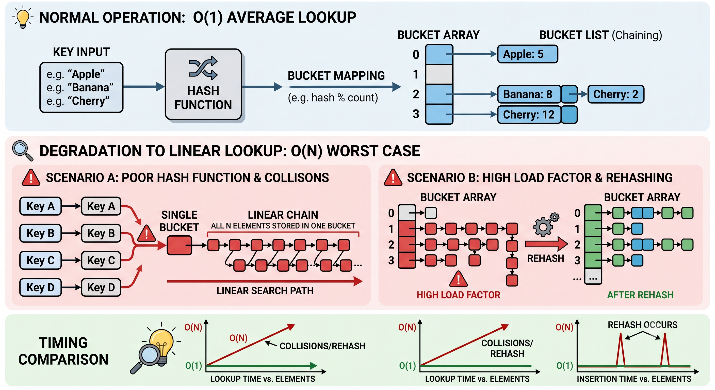
The Problem of Collisions

No hash function is perfect.

Different keys can sometimes produce the same bucket index.

Example:

Key A -> Bucket 4

Key B -> Bucket 4

Key C -> Bucket 4

This situation is called a collision.

---

How Does unordered_map Handle Collisions?

Most standard library implementations use Separate Chaining.

Instead of storing only one element per bucket, each bucket stores a linked list (or a similar node-based structure).

Example:

Bucket 4

↓

[Alice]

↓

[Bob]

↓

[Charlie]

↓

nullptr

When searching,

1. compute the bucket
2. traverse only that bucket’s chain
3. compare keys

Even if three elements exist in the bucket, that’s still much faster than searching the entire table.

---

Visualizing Separate Chaining

Bucket 0

nullptr

---------------------

Bucket 1

[John]

↓

[Mike]

↓

nullptr

---------------------

Bucket 2

nullptr

---------------------

Bucket 3

[Alice]

↓

[Bob]

↓

[David]

↓

nullptr

Every node stores

• key
• value
• hash (sometimes cached by implementations)
• pointer to next node

Conceptually,

struct Node
{
    Key key;
    Value value;
    Node* next;
};

---

Why Doesn’t Performance Always Stay O(1)?

Suppose every key lands in the same bucket.

Bucket 0

A

↓

B

↓

C

↓

D

↓

E

↓

F

Searching now becomes

A

↓

B

↓

C

↓

D

↓

E

This is essentially a linked list search.

Time complexity becomes

O(n)

This is the worst-case scenario.

Fortunately, good hash functions make this extremely unlikely for typical workloads.

---

Load Factor

The hash table keeps track of how full it is.

Load Factor is defined as

Load Factor = Number of Elements / Number of Buckets

Example

80 elements

40 buckets

Load Factor = 2.0

Higher load factor means

• more collisions
• longer chains
• slower lookups

---

Rehashing

When the load factor becomes too large, the hash table expands itself.

Suppose initially

Buckets = 8

After many insertions,

Buckets = 16

Every element is hashed again because

hash % 8

is different from

hash % 16

So every node must be moved into its new bucket.

Old Table

Bucket 3

Alice

↓

Bob

↓

Charlie

After rehashing

Bucket 5

Alice

-----------------

Bucket 11

Bob

-----------------

Bucket 2

Charlie

Notice how collisions often decrease after rehashing.

---

Why is Rehashing Expensive?

Rehashing requires

• allocating a larger bucket array
• recomputing bucket indices
• moving every node
• updating bucket pointers

That makes a single rehash operation O(n).

However, it happens infrequently.

Because the cost is spread across many insertions, the average insertion complexity still remains O(1).

This concept is known as amortized constant time.

---

Custom Hash Functions

Not every type has a built-in hash function.

Suppose we have

struct Point
{
    int x;
    int y;
};

Using it directly won’t compile because the standard library doesn’t know how to hash it.

We can define our own hash.

struct PointHash
{
    size_t operator()(const Point& p) const
    {
        return hash<int>()(p.x) ^ (hash<int>()(p.y) << 1);
    }
};

Now,

unordered_map<Point, string, PointHash> mp;

works as expected (assuming operator== is also defined for Point).

---

Memory Layout (Conceptually)

Bucket Array

+----+      +--------+
| 0  | ---> | Node   |
+----+      +--------+
| 1  | ---> nullptr
+----+
| 2  | ---> | Node |
|             |
|             v
|          | Node |
+----+
| 3  | ---> nullptr
+----+

Notice that

• buckets are contiguous
• nodes are individually allocated
• nodes are connected through pointers

This explains why unordered_map generally uses more memory than a vector.

---

unordered_map vs map

Feature	unordered_map	map
Internal Structure	Hash Table	Balanced Binary Search Tree (typically Red-Black Tree)
Lookup	Average O(1)	O(log n)
Insertion	Average O(1)	O(log n)
Deletion	Average O(1)	O(log n)
Worst Case	O(n)	O(log n)
Order Maintained	No	Yes
Iterator Order	Unspecified	Sorted by Key
Memory Usage	Usually Higher	Usually Lower per element, but tree pointers still add overhead

If your application doesn’t require sorted keys, unordered_map is often the better choice for raw lookup performance.

---

Common Mistakes

1. Assuming iteration order is fixed

unordered_map<int, int> mp;

The iteration order is not guaranteed and may change after insertions or rehashing.

---

2. Ignoring poor hash functions

A weak custom hash function can cause many collisions, degrading performance significantly.

---

3. Forgetting about rehashing

Pointers, references, or iterators may become invalid after a rehash. If your code stores iterators for long periods, be aware that insertions triggering rehashing can invalidate them.

---

4. Using operator[] for lookups

mp[key];

If key doesn’t exist, this creates a new element with a default-constructed value.

If you only want to check for existence, prefer

mp.find(key)

or, in C++20 and later,

mp.contains(key)

---

Complexity Summary

Operation	Average	Worst Case
Insert	O(1)	O(n)
Search	O(1)	O(n)
Delete	O(1)	O(n)
Rehash	O(n)	O(n)

The average-case performance assumes:

• A good hash function.
• A reasonable load factor.
• Well-distributed keys.

---

Final Thoughts

std::unordered_map achieves its impressive performance by combining three key ideas: hashing, buckets, and collision handling. A hash function maps keys to buckets, separate chaining resolves collisions, and periodic rehashing keeps the table efficient as it grows.

While the implementation details vary between standard library vendors such as GCC’s libstdc++, LLVM’s libc++, and Microsoft’s STL, the underlying concepts remain the same. Understanding these internals not only helps you use unordered_map more effectively but also makes it easier to reason about performance, choose appropriate data structures, and design better hash functions for custom types.

The next time you write unordered_map<Key, Value>, you’ll know that behind the simple interface is a carefully engineered hash table balancing speed, memory usage, and scalability.